Calculus with analytic geometry II

Contents

1 Integration by parts

2 Trigonometric integrals

3 Trigonometric substitution

4 Partial fraction decomposition

5 Summary of integration techniques

6 Improper integrals

7 Arc length and area of surfaces of revolution

8 Applications to physics

9 Separable differential equations

10 Approximate methods for integrals and differential equations

11 Parametric curves

14 The integral convergence test

15 Comparison tests

16 Alternating series

17 Absolute convergence, root and ratio tests

18 Definition and basic properties of power series

19 Representing functions by power series

Bonus: A relation between power series and differential equations

20 Taylor and Maclaurin series

21 Approximating functions with Taylor polynomials

22 Polar coordinates and applications

23 Conic sections

#	Topics	Links to video
0.0	Welcome video

Integration by parts

#	Topics	Links to video
1	*Notes on integration by parts*
1.1	Integration by parts: motivation and formula
1.2	Integrating \( x \sin x\) and the choice of \( u \)
1.3	How to not integrate \(x \sin x\) Do not repeat at home
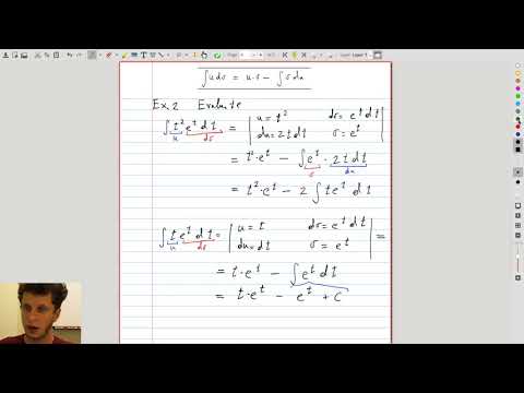
1.4	Getting rid of the second power of \( t\) by integrating by parts Do repeat at home (twice)
1.5	Integrating inverse functions and definite integrals by parts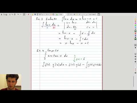
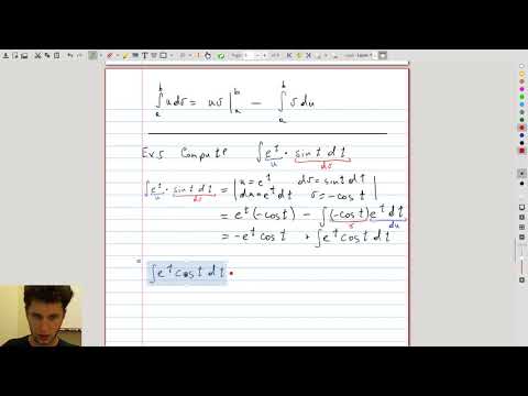
1.6	Integration by parts with moving terms to the other side In this example, we repeatedly integrate by parts and move some of the terms around to arrive at the answer
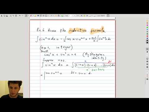
1.7	We obtain the reduction formula for \(\sin x\) This example shows how trig identities will be useful for integration, and prepares us for the next section

Trigonometric integrals

#	Topics	Links to video
2	*Notes on trigonometric integrals*
2.1	What is a trigonometric integral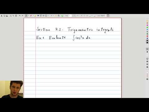
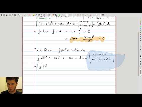
2.2	We integrate \(\sin^5 x \, \cos^2 x \) What is common to these products so far?
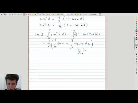
2.3	Applying half-angle formulas After realizing that the previous examples contain odd degrees of \(\sin, \cos\), we discuss dealing with even powers
2.4	In order to integrate \(\sin^4 x\), half-angle formulas have to be applied repeatedly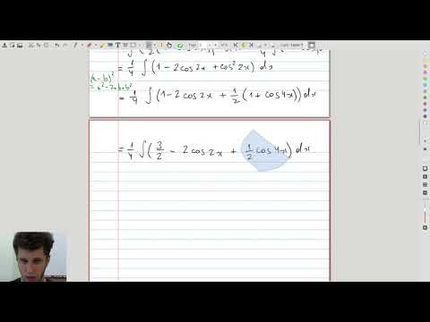
2.5	The above examples are summarized into a general strategy for integrating products of \(\sin x\) and \(\cos x\)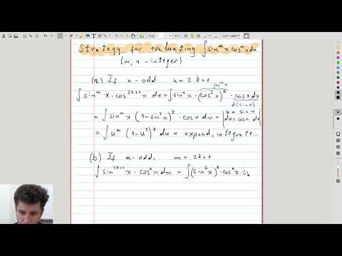
2.6	What is essential about our integration strategy? Why does it work?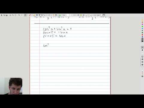
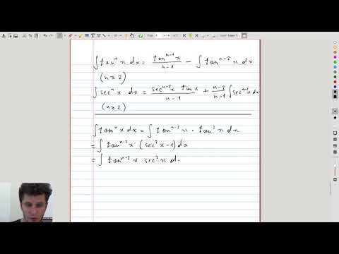
2.7	Examples of integrating products of \(\tan x\) and \(\sec x\)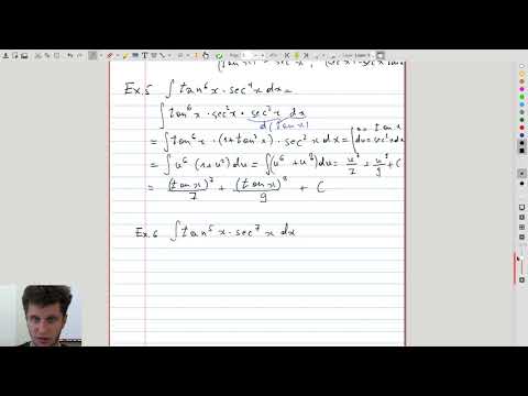
2.8	A general strategy for products of \(\tan x\) and \(\sec x\) is obtained in this video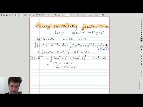
2.9	Some special cases not covered by the strategy for \(\tan x\) and \(\sec x\) Some products of \(\tan x\) and \(\sec x\) are still not covered by our general strategy. This video discusses how to use the Pythagorean identity and integration by parts to obtain reduction formulas for such cases, not covered previously.

Trigonometric substitution

#	Topics	Links to video
3	*Notes on trigonometric substitution*
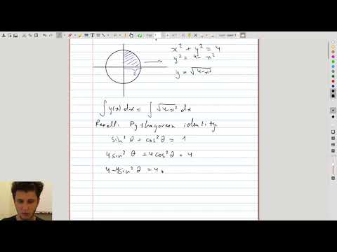
3.1	Motivation for trig sub Evidence that trig sub shows up in some natural integrals.
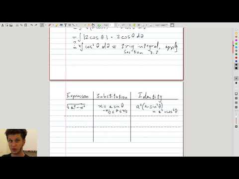
3.2	Main table of trigonometric substitutions We summarize the motivational examples into a table of different trig subs and identities that explain them.
3.3	Substituting \(x = a \sin\theta\)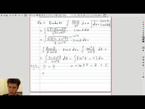
3.4	Substituting \(x = a \sec\theta\)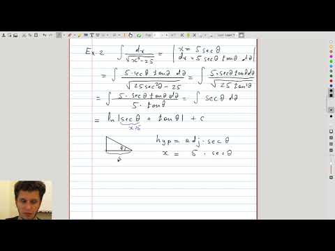
3.5	Definite integrals with trig sub and handling coefficients on \(x^2\) Instead of \(\pm x^2 \pm a^2\) under the radical, in this example we have \(\pm c^2 x^2 \pm a^2\). We show how to factor out the coefficient at \(x^2\) from the integral.
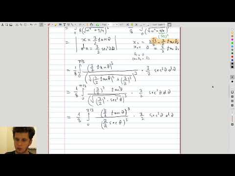3.6	Completing the square to apply a trig sub In this example, expression under the square root is not of the form \(\pm x^2 \pm a^2\), but instead a complete quadratic polynomial. We show how to reduce it to the standard form.

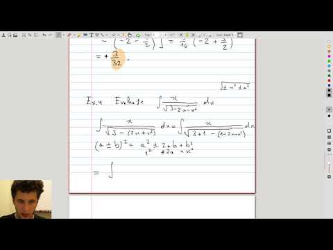Partial fractions

#	Topics	Links to video
4	*Notes on partial fraction decomposition*
4.1	Motivation for partial fraction decomposition Definition of a rational function and the general idea of partial fraction decomposition
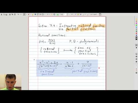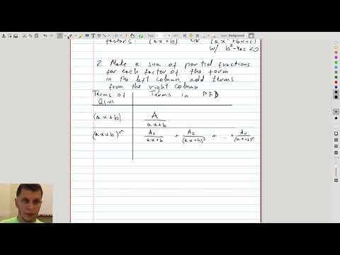
4.2	Main table of partial fraction decomposition An overview of the algorithm for partial fraction decomposition and a table for the partial fractions corresponding to different irreducible factors in denominator.
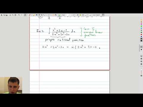
4.3	Long division and unique linear factors We use long division to split an improper rational function into a sum of a polynomial with a proper part. In the second example, we integrate a rational function with unique (nonrepeated) factors in the denominator.
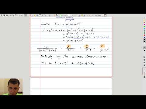
4.4	Repeated linear factors An example of a rational function with repeated linear factors in the denominator. We determine the coefficient by equating the coefficients for the powers of \(x\).
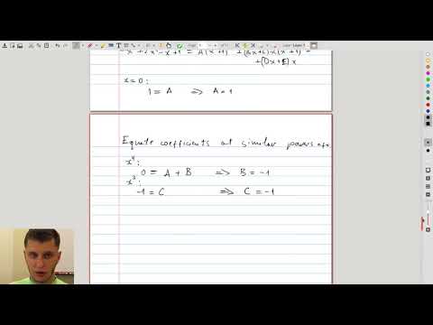
4.5	Unique quadratic factors Integration of a rational function with unique (nonrepeated) irreducible quadratic terms.
4.6	Repeated quadratic factors Integration of functions with repeated irreducible quadratic terms. In particular, we see how to apply trig sub to negative powers of \(1+x^2\).
4.7	Completing a square in a partial fraction We demonstrate how to integrate a partial fraction with an irreducible quadratic factor by completing a square, and applying a u-sub.
4.8	Rationalizing substitution When integrating an expression with an n-th order root, we introduce a u-sub equal to this root, and reduce the problem to integration of a rational function.

Summary of integration techniques

#	Topics	Links to video
5	*Notes on the integration strategy*
5.1	An overview of integration heuristics
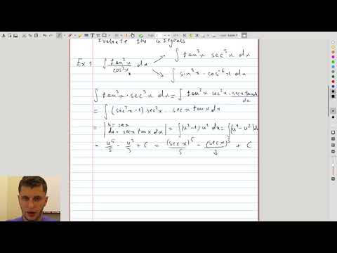
5.2	Examples 1-2 These examples illustrate simplification of the integrand before integration and combining two different techniques: u-sub and integration by parts.
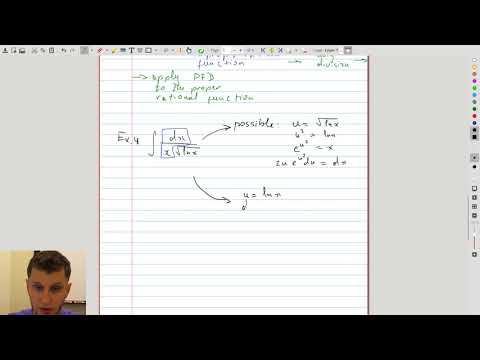
5.3	Examples 3-5 A discussion of the PFD and the usefulness of algebraic transformations, such as multiplying by the conjugate expression.
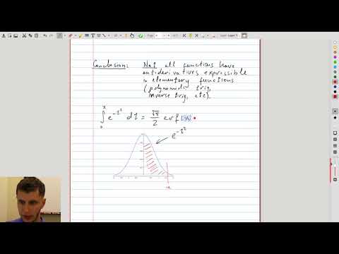
5.4	Conclusion: not all expressions have antiderivatives in elementary functions Our course just scratches the surface of the vast functional universe. The antiderivatives of some of its inhabitants can only be expressed through special functions (error function, Bessel functions, etc), others don’t have a nice representation at all.

Improper integrals

#	Topics	Links to video
6	*Notes on improper integrals*
6.1	Definition of an improper integral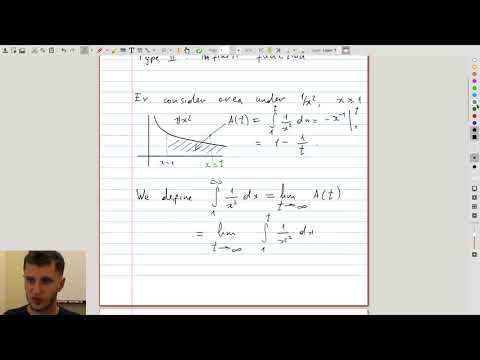
6.2	Convergence of the integral of \(1/x^p\) for different values of \(p\)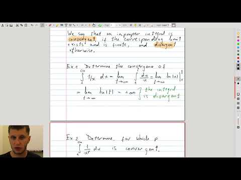
6.3	Using integration by parts in improper integrals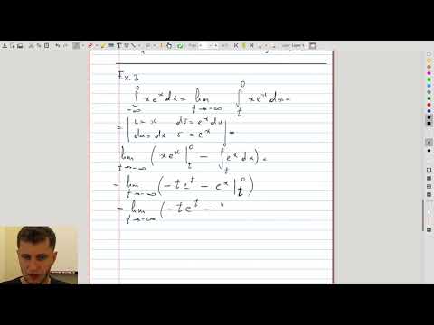
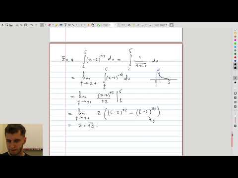
6.4	Improper integrals of type II and the comparison theorem Improper integrals of the second type contain a function that becomes infinite at some point of the integration interval. We also discuss the comparison theorem and see its application to integral of \(e^{-x^2}\). Specifically, even though this function does not have an antiderivative in elementary functions, we are able to determine that its improper integral converges.

Arc length and area of surfaces of revolution

#	Topics	Links to video
7	*Notes on arc length*
7.1	Derivation of the formula for the arc length of a curve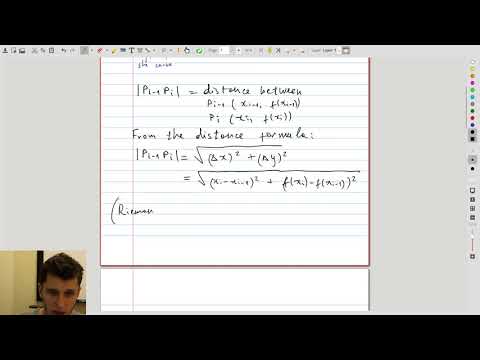
7.2	First example: length of the curve \(y^2 = x^3\)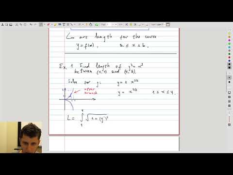
7.3	Treating a curve as the graph of \(x = x(y)\)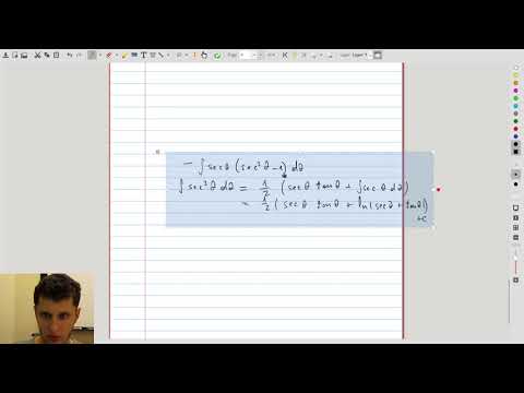
7.4	The arc length function: definition and use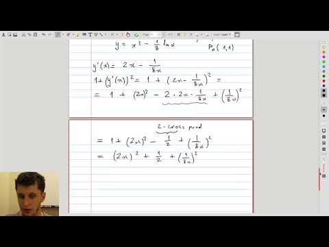
7.5	Summary of arc length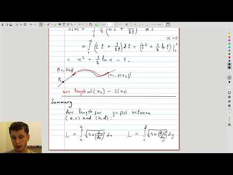
	*Notes on areas of surfaces of revolution*
7.6	Derivation of the formula for the area of surface of revolution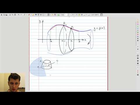
7.7	Area of a spherical slice and using cylindrical projection in cartography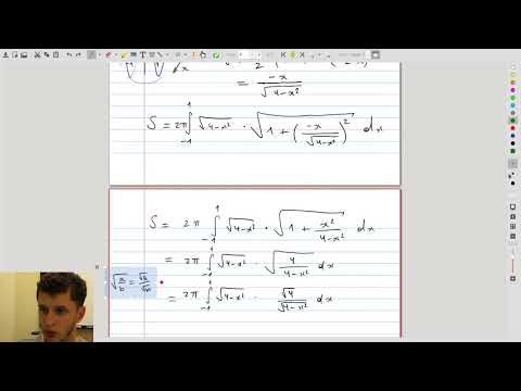
7.8	Rotation of an arc of \(y=x^2\). Solved two ways: integrating in \(x\) and in \(y\). The variable of integration is independent of the axis.
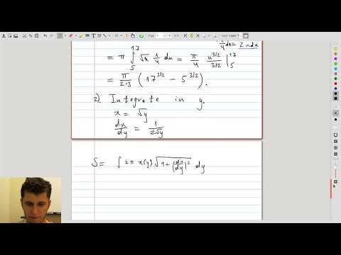7.9	Summary: how to set up the integral for a surface of revolution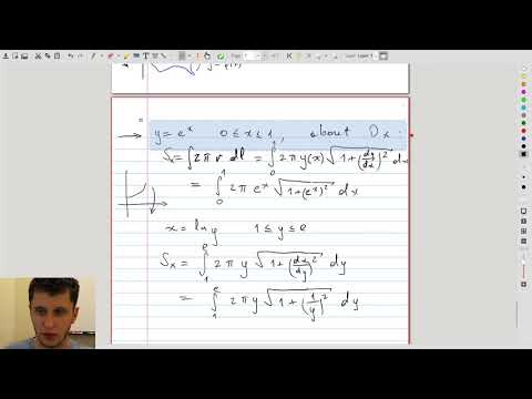

Applications to physics

#	Topics	Links to video
8	*Notes on applications to physics*
8.1	Hydrostatic force: derivation and example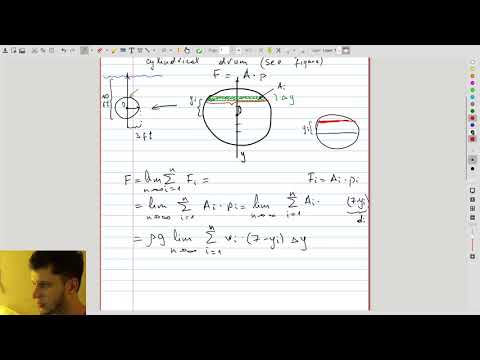
8.2	Center of mass of a region: formula and example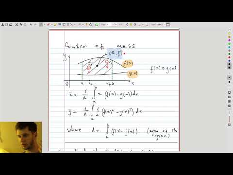

Separable differential equations

#	Topics	Links to video
9	*Notes on differential equations*
9.1	Introduction: why we care about integration techniques and an outline of the solution process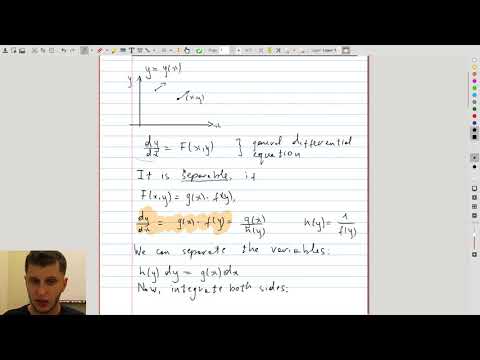
9.2	Applying the initial condition to select a specific solution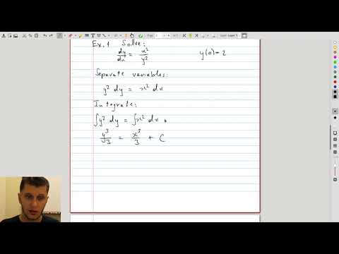
9.3	When solving for \(y\) can be tricky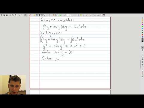
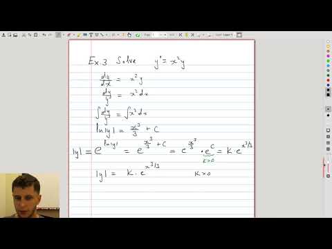
9.4	Absorb \(\pm\) into the positive constant, by extending the range of admissible constants This is useful when solutions have the form \(\|y\| = K e^x, \ K >0 \).
9.5	Modeling a simple electric circuit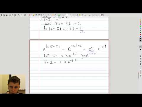
9.6	Mixing problems A common class of problems which involve uniform mixing of a solution.
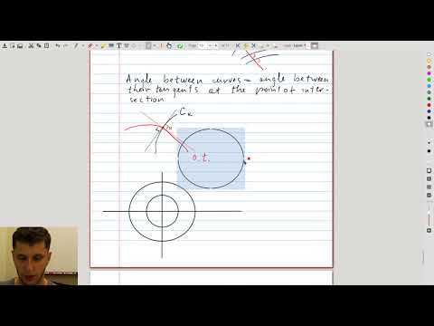
9.7	Orthogonal trajectories These generalize both Cartesian and polar coordinates. Imagine curved coordinate lines!

Approximate methods for integrals and differential equations

#	Topics	Links to video
10	*Notes on approximate methods* To run the examples discussed in SageMath videos interactively from your browser, follow this link. More information about Sage can be found on the course page.
10.1	Introduction: when it is necessary to solve an integral or a differential equation approximately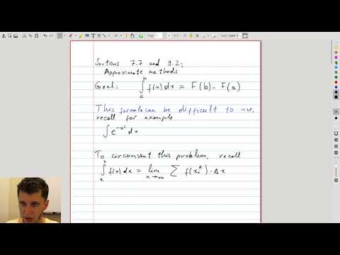
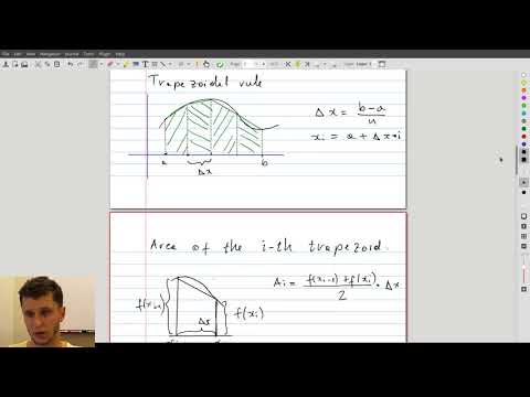
10.2	Derivation of the midpoint and trapezoidal rules These rules are obtained by approximating area under the curve with rectangles and trapezoids, respectively.
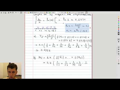
10.3	Trapezoidal vs midpoint rule: which is better? See if you favorite is a more precise rule!
10.4	Error bounds for \(T_n\) and \(M_n\)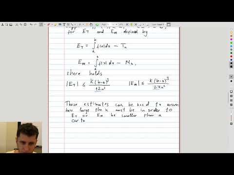
10.5	Simpson’s rule and its error bound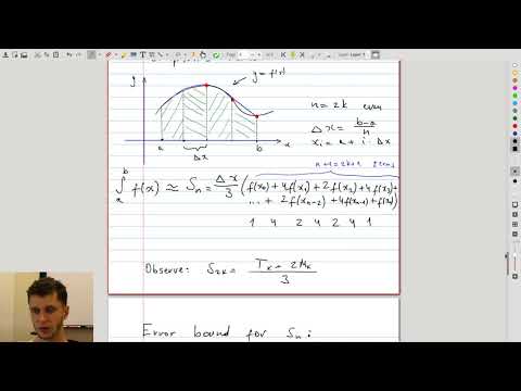
10.6	Numerical integration in SageMath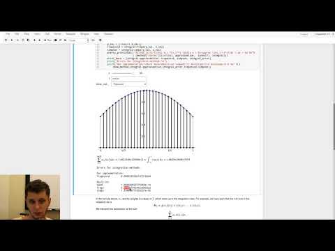
10.7	Euler’s method This video discusses how to view a differential equation as a vector field, by attaching a little vector to every point of the \(x,y\) plane, and how to construct approximate solutions by connecting the points obtained from Euler’s method.
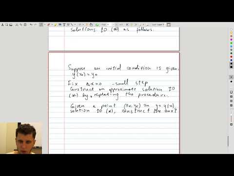10.8	Euler’s method in SageMath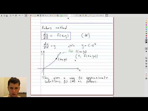

Parametric curves

#	Topics	Links to video
11	*Notes on parametric curves*
11.1	The definition of the parametric curve. Curve as a trajectory of motion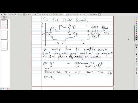
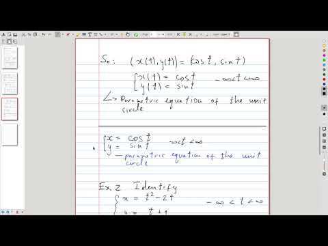
11.2	Parameter elimination technique We introduce the primary technique for expressing a parametric curve as a regular curve: by eliminating the parameter \(t\). This technique is used to identify a parametric curve.
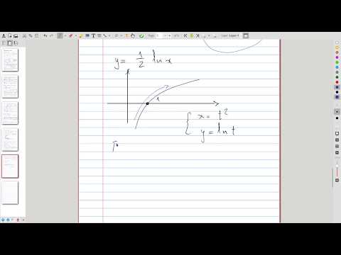
11.3	The parametric curve \( (x(t),\, y(t)) = (t^2, \ln t) \) We show that every parametric curve has two characteristics: the shape and the direction of motion of a particle along this shape. Plus, in this example we get to reverse time Dr. Who-style 😮
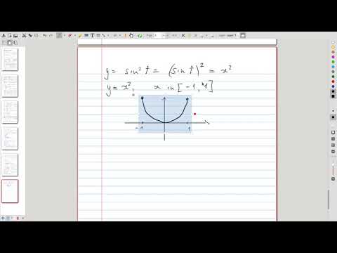
11.4	The parametric curve \( (x(t),\, y(t)) = (\sin t, \sin^2 t) \) A piece of parabola along which we oscillate back and forth
11.5	The parametric curve \( (x(t),\, y(t)) = (\tan^2\theta, \sec \theta ) \), which shows that the range of the parameter is important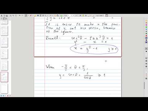
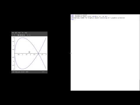
11.6	Tangents to parametric curve We look at a self-intersecting curve, which has not one, but two tangents at the same point! (and does not pass the vertical line test) Link to SageMath.
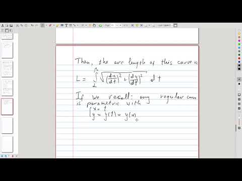
11.7	Computing arc length of parametric curves The formula and an example: length of a circle
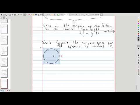
11.8	Area of surfaces of revolution for parametric curves The formula and an example: area of a sphere

Sequences

#	Topics	Links to video
12	*Notes on sequences*
12.1	Definition of a sequence and some generic examples: populations, digits of \(e\), etc.
12.2	Limits of sequences and limit laws
12.3	Lifting to functions: to apply l’Hôpital’s rule, pass to the function first!
12.4	Interchanging limits with continuous functions
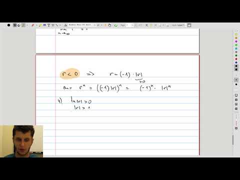
12.5	When is the sequence \(r^n\) convergent? This will be useful later, when we discuss the geometric series.
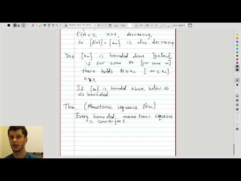
12.6	Monotonic sequences We discuss increasing and decreasing sequences, and a theorem about them. This theorem will be used for establishing convergence of series with nonnegative terms.

Series

#	Topics	Links to video
13	*Notes on series*
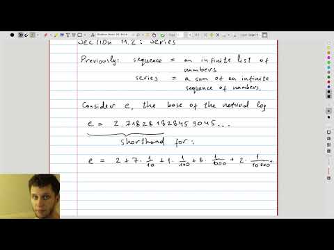
13.1	Definition of a series and its sum Any decimal expansion is an example of number series!
13.2	The first example; finding \(a_k\) through \(s_n\)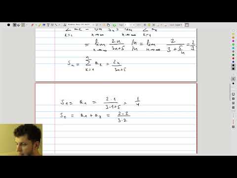
13.3	Telescoping series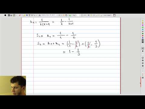
13.4	Geometric series: condition of convergence and sum formula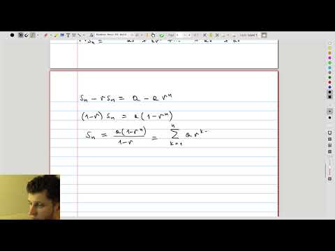
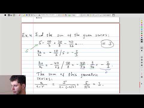
13.5	Examples of geometric series How to recognize a geometric series and evaluate its sum
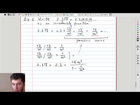
13.6	Rewriting a number with periodic decimal expansion as a fraction If the decimal expansion of a number is periodic, it can be represented as an irreducible fraction. In this example, we show how. (In contrast, say, \(\sqrt 2\) or \(\pi\) have decimal expansions that are not periodic.)
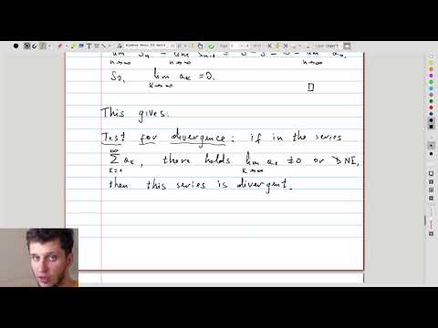
13.7	Test for divergence and the harmonic series If the terms of a series \(a_k\) do not converge to 0, this series is divergent (does not have a finite sum). The converse is not true: if \( a_k \to 0,\ k\to \infty \), their sum \(\sum_k a_k\) is not necessarily convergent. An example of such series is \(\sum_k \frac 1k \). Clearly \(1/k \to 0,\ k\to \infty\), and yet the series diverges.
13.8	A short illustration of how the test for divergence is applied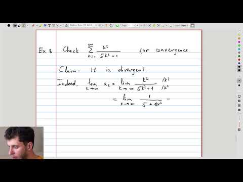
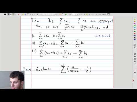
13.9	Arithmetic operations with series The limit laws enable adding limits and multiplying them by constants. Because the sum of a series is the limit of its partial sums, the limit laws for addition and subtraction extend to series.
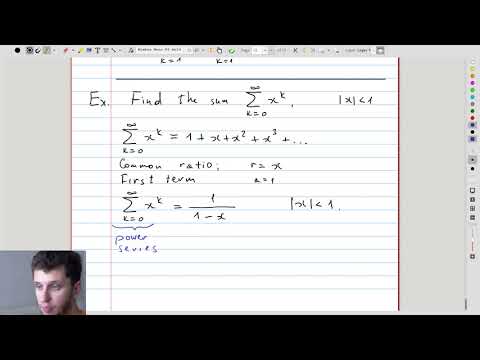
13.10	A glimpse of power series As a sneak peek into what we will discuss next, we obtain an expansion of \(\frac1{1-x}\) into a power series. 😱

Integral test

#	Topics	Links to video
14	*Notes on the integral test*
14.1	Showing that \(\sum_{k} \frac1{k^2} \) is convergent, using integrals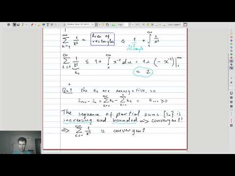
14.2	Showing that \(\sum_k \frac1{k^{1/2}} \) is divergent and the statement of the integral test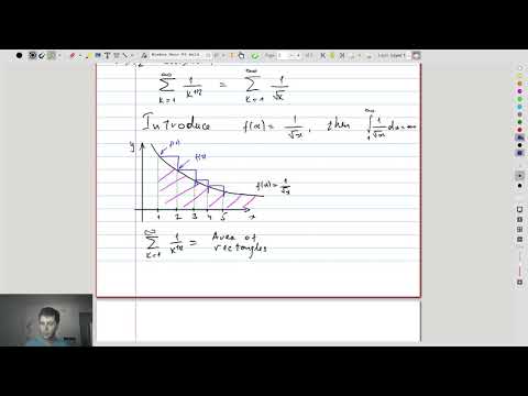
14.3	Convergence of \(\sum_k \frac1{k^{2}+1} \)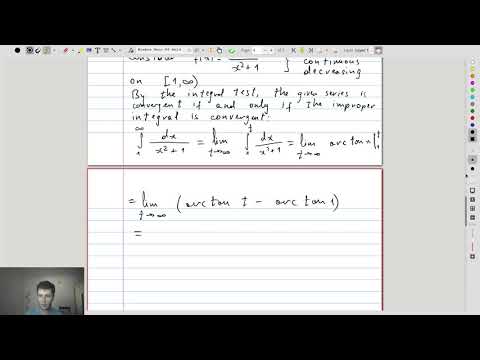
14.4	For which \(p\) is \(\sum_k \frac1{k^{p}} \) convergent? (For \(p>1\), just as improper integrals.)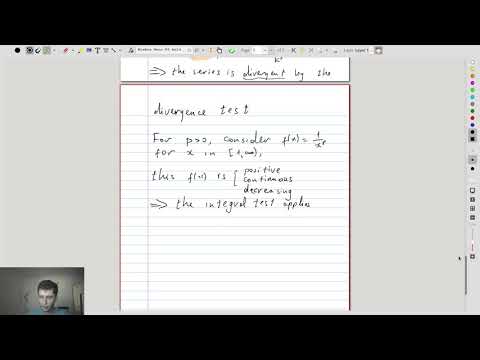
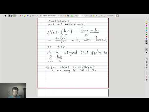
14.5	Convergence of \(\sum_k \frac{\ln k}{k} \) In order to show that \(f(x) = \ln(x)/x\) is decreasing, we have to compute its derivative. It turns out, the function is decreasing only for \(x>e\), but we can still apply the integral test.
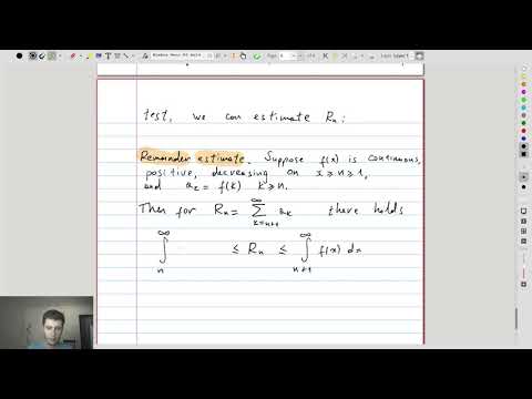
14.6	Formulation of the remainder estimate Using the ideas from integral test, we estimate the n-th remainder, \(R_n = s - s_n\) for a series \(\sum_k a_k \), converging to the finite value \(s\).
14.7	Applying the remainder estimate to the series \(\sum_k \frac1{k^3}\)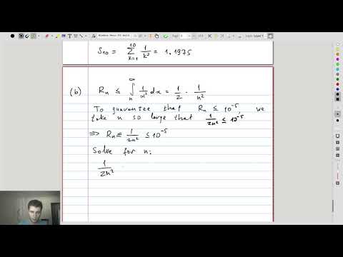

Comparison tests

#	Topics	Links to video
15	*Notes on the comparison tests*
15.1	The statement of the comparison test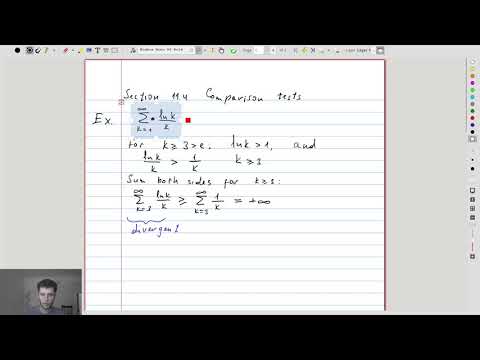
15.2	Applying the comparison test: compare a given series to geometric and p-series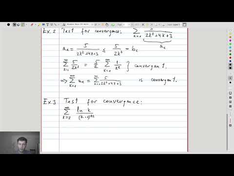
15.3	Limit comparison test If obtaining an inequality comparing \(a_k\) and \(b_k\) is difficult, it is useful to consider the limit of their ratio: \(\lim_{k\to\infty} \frac{a_k}{b_k} \)

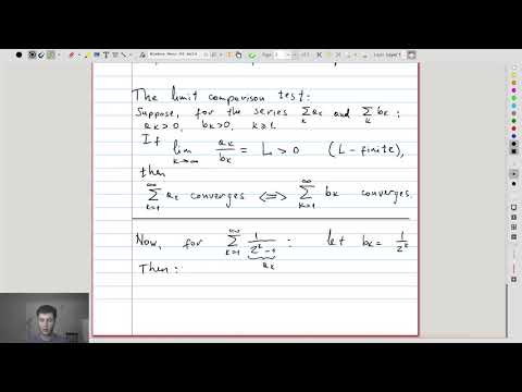Alternating series

#	Topics	Links to video
16	*Notes on alternating series*
16.1	Definition of alternating series and statement of the alternating series test
16.2	Applying the alternating series test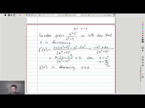

Absolute convergence, root and ratio tests

#	Topics	Links to video
17	*Notes on absolute convergence, root and ratio tests*
17.1	The notion of absolute convergence Absolute convergence allows to bypass the specifics of signs of \(a_k\) in a series \(\sum_k a_k\), and only look at the series of absolute values \(\sum_k \|a_k\| \). Then convergence of this series of absolute values implies usual convergence of the original series \(\sum_k a_k\).
17.2	Application of absolute convergence to the series \(\sum_k \frac{\cos k}{k^2} \)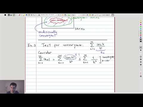
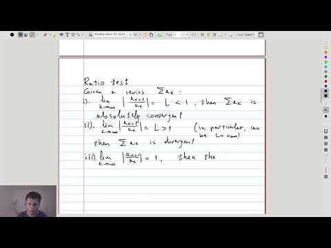
17.3	The ratio test: statement Especially suitable for expressions containing e.g. \(a^k\) and \(k!\).
17.4	Ratio test applied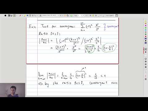
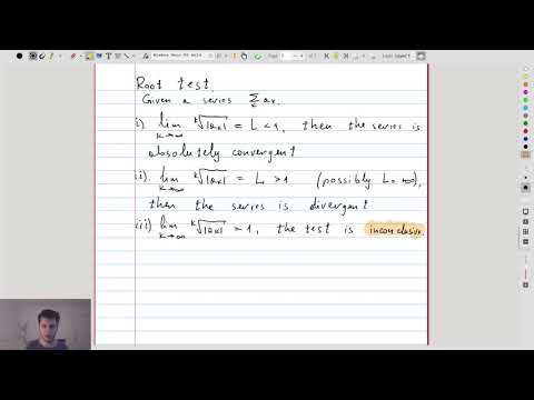
17.5	The root test: statement and an example Especially suitable for \(a_k = (some\ expression)^k\).

Power series

#	Topics	Links to video
18	*Notes on power series*
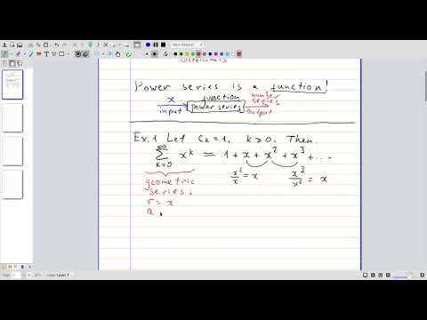
18.1	Definition of power series The image quality is not great, and the colors are inverted. This has been corrected in subsequent videos
18.2	Find the values of \(x\) that make the power series \(\sum_k \frac{(x-3)^k}k\) converge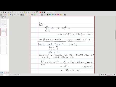
18.3	Finding the regions of convergence for \(\sum_k k!x^k \) and the Bessel function \( J_0 \)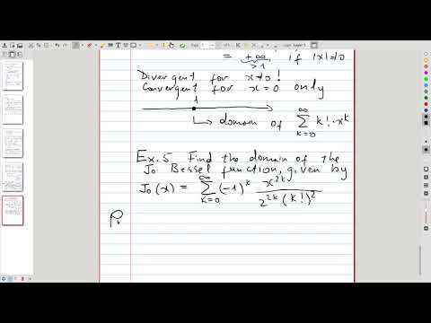
18.4	We explore the graph of the Bessel function \( J_0 \)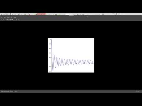
18.5	Summary of different convergence modes for power series.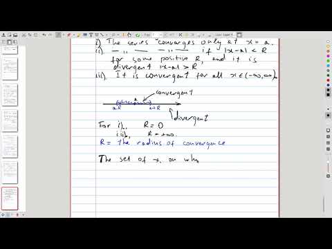
18.6	Using the theorem from 1.5, we determine the interval of convergence (= all the values of \(x\) for which it converges) for the series \( \sum_k \frac{(-3)^k x^k}{\sqrt{k+1}} \).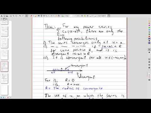

Representing functions by power series

#	Topics	Links to video
19	*Notes on representing functions by power series*
19.1	Representing functions with power series using algebraic manipulations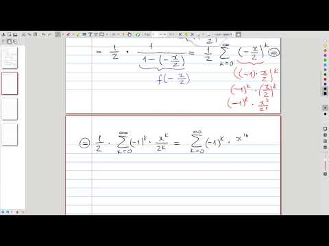
19.2	The main theorem concerning differentiation and integration of power series, and an example that involves differentiating a series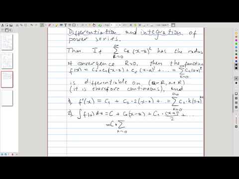
19.3	A comment on changing indexing in a series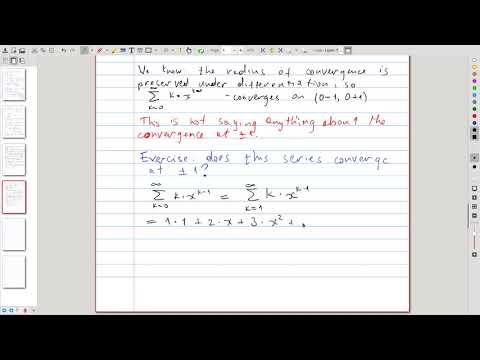
19.4	Two important examples: power series for \(\ln(1+x)\) and \(\arctan x\)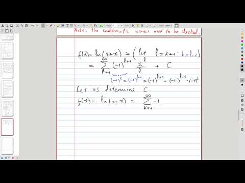
19.5	Discussion of the series for \(\ln(1+x)\) and \(\arctan x\)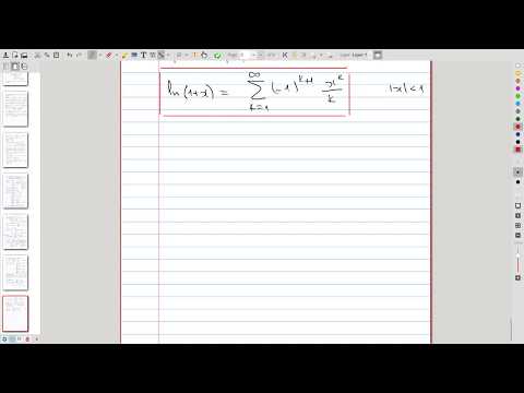
19.6	Representing an antiderivative of a function by the power series, and why it is useful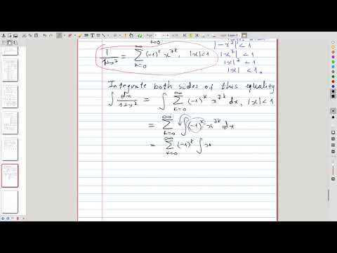

Bonus: A relation between power series and differential equations

#	Topics	Links to video
	*A relation between power series and differential equations.*
	Connecting two major topics of this course, we solve the homework question #8 from section 11.9. First, we show that the power series \(f(x) = \sum_{n=0}^\infty \frac{x^n}{n!} \) satisfies the differential equation \(f’(x)=f(x)\). Then, we solve this differential equation and verify that its unique solution with the initial condition \(f(0)=1\) is \(e^x\). This gives an alternative way to compute the power series representation for \(e^x\).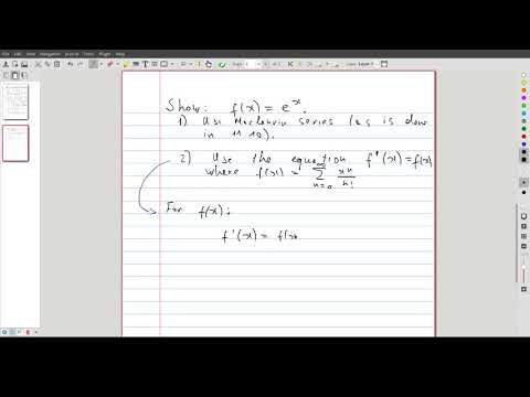

Taylor and Maclaurin series

#	Topics	Links to video
20	*Notes on Taylor and Maclaurin series*
20.1	The main theorem about Taylor series is discussed, which gives the expressions for the coefficients in the Taylor series of a function through its derivatives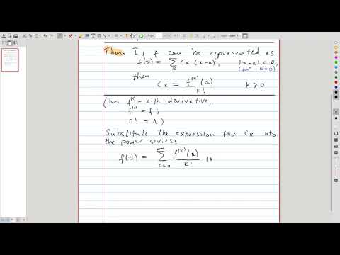
20.2	Computing the Maclaurin series for \(e^x\)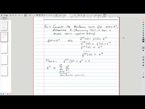
20.3	How to prove that Taylor series of a function converges to it? We discuss the remainder estimate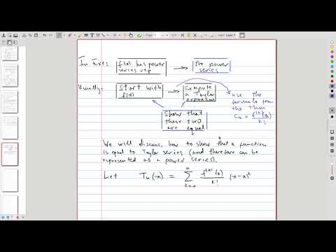
20.4	Using the remainder estimate, we show that the Maclaurin series for \(e^x\) converges to it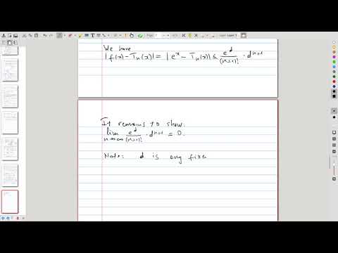
20.5	Maclaurin series for \(\sin x\)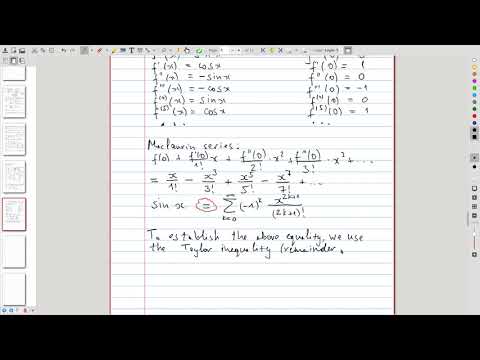
20.6	Using the previous example, we calculate the Maclaurin expansion for \(\cos x\)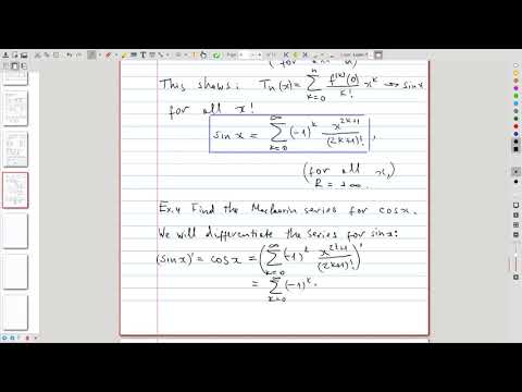
20.7	We apply algebraic manipulations to the series for \(\cos x\) in order to compute the Maclaurin series of \(x \cos(x^3)\) and its radius of convergence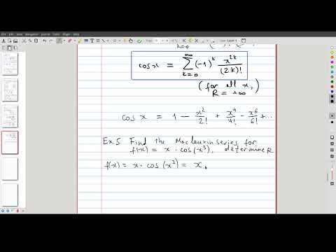
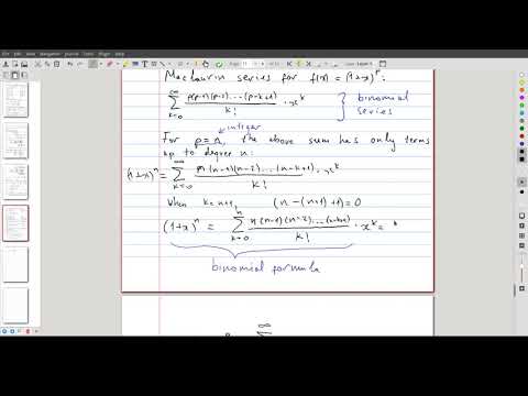
20.8	The binomial series: expansion of \((1+x)^p\) For more context about binomial coefficients arising in polynomials, read this note.
20.9	Proof of the main theorem about Taylor series from 19.1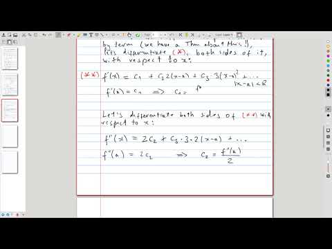

	*Notes on examples and applications of Taylor and Maclaurin series*
20.10	We consider an application of the binomial series formula, obtaining the Maclaurin expansion for \(\frac1{\sqrt{4-x}}\)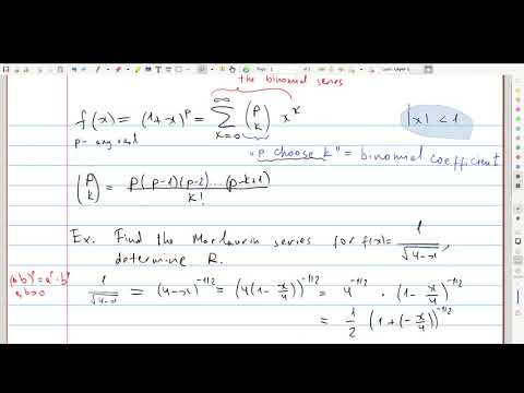
20.11	An example of computing a Taylor series — the expansion of \(\sin x\) around the center \(a = \frac{\pi}{3}\)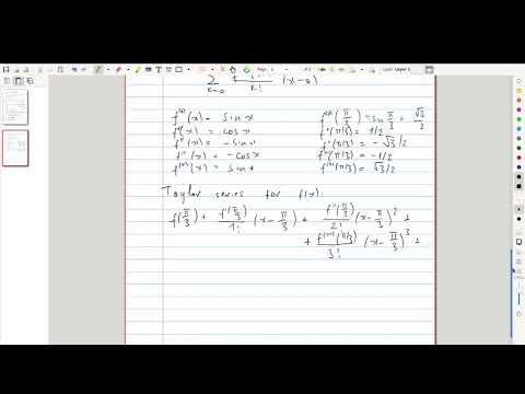
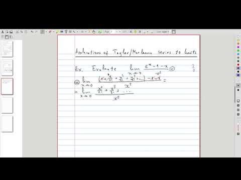
20.12	Using power series to compute limits Turns out, not only power series can be used to approximate functions and compute antiderivatives, you can also use them instead of l’Hôpital’s rule to evaluate limits!
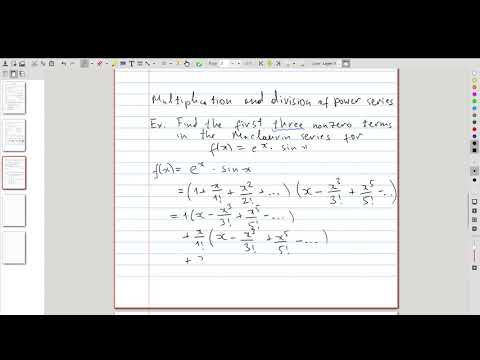
20.13	Example of multiplying two power series We mentioned earlier that power series were the closest thing to infinite polynomials. In this video we show they are in fact so close to polynomials, one can multiply two power series together!
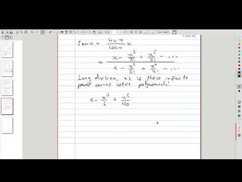
20.14	Division of power series If the previous video was somewhat surprising, this one is nothing short of astounding. We will perform long division on infinite series, just like as if they were polynomials 😮

Approximating functions with Taylor polynomials

#	Topics	Links to video
21	*Notes on approximation with Taylor polynomials*
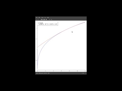
21.1	Approximating \( \sqrt[3]x\) close to the point \(a = 8\) with \(T_2(x)\), and estimating the resulting error We discuss a typical application of Taylor series — approximation of a function close to a point where its value is known. This is how Taylor series usually show up in computational applications.
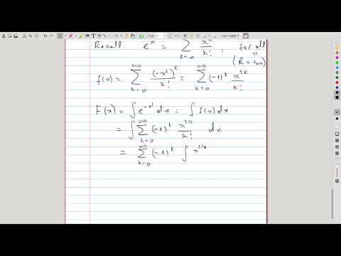
21.2	Antiderivative of \( e^{-x^2} \) The antiderivative of \( e^{-x^2} \) cannot be expressed in terms of elementary functions. It can, however, be represented by a (Maclaurin) power series converging everywhere. We obtain such representation, demonstrating the expressiveness of power series.
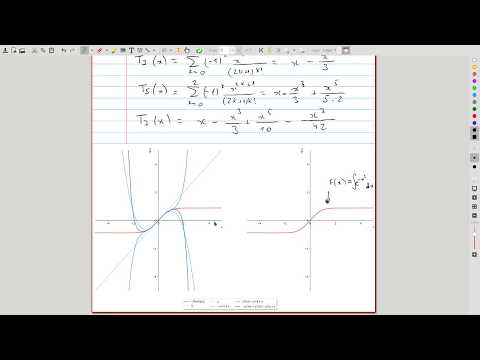
20.3	Comparison of the initial Taylor polynomials We plot the function from episode 20.2 alongside several of its Taylor polynomials and discuss the code of the Python routine used to produce these graphs.

Polar coordinates and applications

#	Topics	Links to video
22	*Notes on polar coordinates and applications*
22.1	Definition of the polar coordinate system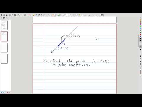
22.2	Conversion formulas: converting between Cartesian and polar coordinates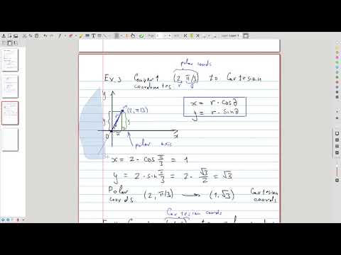
22.3	Polar curves, definition and simple examples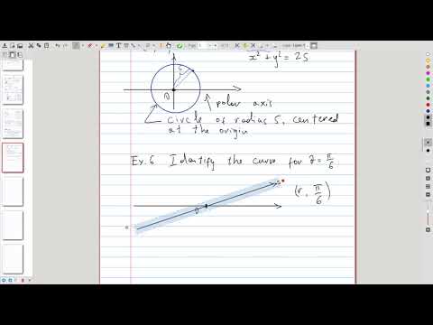
22.4	Sketching polar curves, illustrated for the cardioid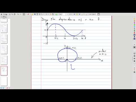
22.5	Polar curves from the parametric perspective We treat polar curves as a special case of parametric curves and establish the formulas for slope and arc length of a polar curve This and the following video suffer from a nasty reverb 😞
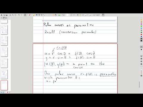22.6	To illustrate arc length formula for polar curves, we evaluate the length of the cardioid, which results in a tricky integral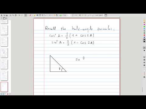
	*Notes on areas in polar coordinates*
22.7	Formula for computing areas in polar coordinates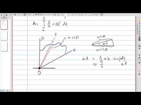
22.8	An example for area in polar coordinates: the region inside the circle \(r = 3\sin \theta\) and outside the cardioid \(r = 1+\sin\theta\)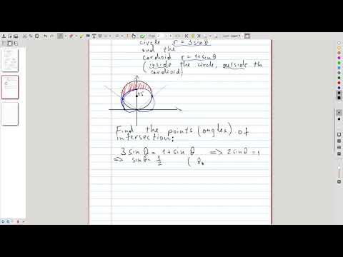

Conic sections

#	Topics	Links to video
23	*Notes on conic sections*
23.1	We discuss various conic sections and show how to obtain them by intersecting the double cone with a plane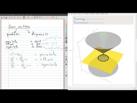
23.2	Parabola: geometric characterization and equation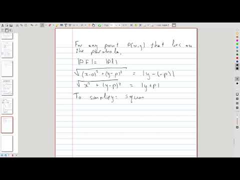
23.3	Ellipse: geometric characterization and equation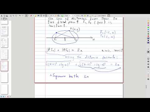
23.4	Hyperbola: geometric characterization and equation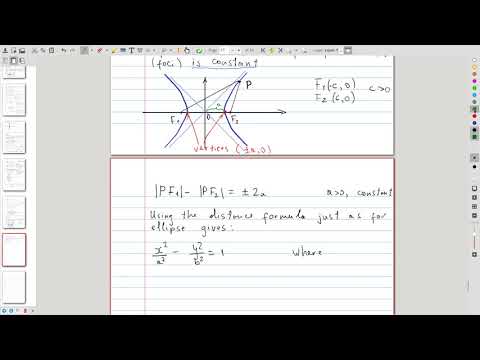