\( \DeclareMathOperator{\abs}{abs} \newcommand{\ensuremath}[1]{\mbox{$#1$}} \)
Using Maxima in Calculus
1 Plotting examples
| --> | plot2d ( sin ( x ) , [ x , 0 , 1 ] ) ; |
| --> | example ( plot3d ) ; |
| --> | plot3d ( x ^ 2 + y ^ 2 , [ x , − 5 , 5 ] , [ y , − 5 , 5 ] , [ gnuplot_pm3d , true ] ) $ |
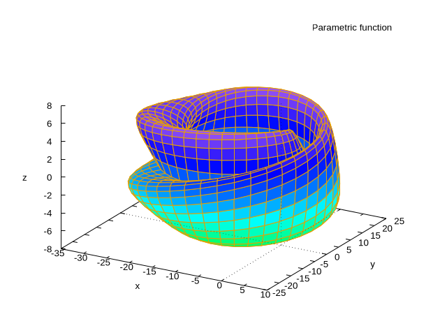
| --> | example ( wxplot3d ) ; |
| (%i1) |
wxplot3d
(
[
5
·
cos
(
x
)
·
(
cos
(
x
/
2
)
·
cos
(
y
)
+
sin
(
x
/
2
)
·
sin
(
2
·
y
)
+
3
.
0
)
−
10
.
0
,
− 5 · sin ( x ) · ( cos ( x / 2 ) · cos ( y ) + sin ( x / 2 ) · sin ( 2 · y ) + 3 . 0 ) , 5 · ( − sin ( x / 2 ) · cos ( y ) + cos ( x / 2 ) · sin ( 2 · y ) ) ] , [ x , − %pi , %pi ] , [ y , − %pi , %pi ] , [ ' grid , 40 , 40 ] ) $ |
\[\tag{%t1} \]
| (%i3) | wxplot2d ( [ atan ( x ) , %pi / 2 , − %pi / 2 ] , [ x , − 10 , 10 ] , [ color , blue , magenta , brown ] ) $ |
\[\tag{%t3} \]
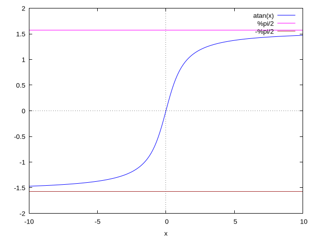
This will display the result in a popup window:
| --> | plot2d ( x ^ 2 · exp ( − x ^ 3 / 1000 ) , [ x , 0 , 20 ] ) $ |
2 Integrate
| --> | integrate ( 1 / ( x + x · sqrt ( x ) ) , x ) ; |
| --> | fullratsimp ( % ) ; |
(% refers to the output of the previous evaluation)
| --> | integrate ( ( 1 − tan ( x ) ^ 2 ) / sec ( x ) ^ 2 , x ) ; |
| --> | trigsimp ( % ) ; |
| --> | integrate ( x ^ 2 / sqrt ( 1 + x ^ 2 ) , x ) ; |
| --> | integrate ( 1 / sqrt ( 16 − x ^ 2 ) ^ 3 , x ) ; |
| --> | integrate ( ( log ( x ) + 5 ) / ( x · ( log ( x ) ^ 2 + 4 ) ) , x ) ; |
3 Find roots of a polynomial
| --> | allroots ( x ^ 10 − 2 · x ^ 4 + 1 / 2 ) ; |
4 Applying "at"
| --> |
Values
:
[
a
=
10
,
c
=
100
]
;
Pyth : a ^ 2 + b ^ 2 = c ^ 2 ; solve ( % , b ) ; result : % [ 2 ] ; at ( result , Values ) ; float ( % ) ; |
| --> |
g1
:
a
·
x
+
y
=
0
;
g2 : b · y + x · x = 1 ; solve ( [ g1 , g2 ] , [ a , b ] ) ; % [ 1 ] ; result_b : b = at ( b , % ) ; |
| --> |
ohm
:
U
=
R
·
I
;
r_parallel : R = R_1 · R_2 / ( R_1 + R_2 ) ; result : at ( ohm , r_parallel ) ; |
| --> | example ( at ) ; |
5 Direction fields
| --> |
plotdf
(
x
−
y
^
2
,
[
xfun
,
"sqrt(x);−sqrt(x)"
]
,
[ trajectory_at , − 1 , 3 ] , [ direction , forward ] , [ y , − 5 , 5 ] , [ x , − 4 , 16 ] ) $ |
| --> |
plotdf
(
[
y
,
−
(
k
·
x
+
c
·
y
+
b
·
x
^
3
)
/
m
]
,
[ parameters , "k=−1,m=1.0,c=0,b=1" ] , [ sliders , "k=−2:2,m=−1:1" ] , [ tstep , 0 . 1 ] ) ; |
| --> |
plotdf
(
[
w
,
−
g
·
sin
(
a
)
/
l
−
b
·
w
/
m
/
l
]
,
[
a
,
w
]
,
[ parameters , "g=9.8,l=0.5,m=0.3,b=0.05" ] , [ trajectory_at , 1 . 05 , − 9 ] , [ tstep , 0 . 01 ] , [ a , − 10 , 2 ] , [ w , − 14 , 14 ] , [ direction , forward ] , [ nsteps , 300 ] , [ sliders , "m=0.1:1" ] , [ versus_t , 1 ] ) $ |
| --> | plotdf ( x ^ 2 · y , [ trajectory_at , . 1 , 1 ] ) $ |
5.1 Examples from class
| --> |
plotdf
(
x
^
2
·
y
,
[ y , − 5 , 5 ] , [ x , − 5 , 5 ] ) $ |
Electric circuit example:
| --> |
plotdf
(
15
−
3
·
y
,
[
xfun
,
"5"
]
,
[ y , − 1 , 10 ] , [ x , − 1 , 10 ] ) $ |
Orthogonal trajectories example:
| --> |
plotdf
(
−
2
·
x
/
y
,
[
xfun
,
"sqrt(x);2·sqrt(x);sqrt(x);3·sqrt(x);−sqrt(x)"
]
,
[ y , − 10 , 10 . 1 ] , [ x , − 10 , 10 ] ) $ |
Tank example:
| --> |
plotdf
(
(
150
−
y
)
/
200
,
[
xfun
,
"150"
]
,
[ y , − 10 , 200 ] , [ x , − 10 , 2000 ] ) $ |
Logistic model:
| --> | plotdf ( 0 . 08 · P · ( 1 − P / 1e3 ) , [ t , P ] , [ P , 0 , 1400 ] , [ t , 0 , 80 ] , [ xfun , "1000" ] ) $ |
Logistic model vs natural growth:
| --> | plot2d ( [ 1000 / ( 1 + 9 · exp ( − 0 . 08 · t ) ) , 1000 , 100 · exp ( 0 . 08 · t ) ] , [ t , 0 , 80 ] , [ y , 0 , 1400 ] , [ color , blue , magenta , red ] , [ style , [ lines , 3 ] ] ) $ |
Logistic model with harvesting:
| --> | plotdf ( 0 . 08 · P · ( 1 − P / 1e3 ) − 35 , [ t , P ] , [ P , 0 , 1400 ] , [ t , 0 , 80 ] , [ xfun , "1000" ] ) $ |
Logistic model with minimal population:
| --> | plotdf ( 0 . 08 · P · ( 1 − P / 1e3 ) · ( 1 − 2e2 / P ) − 5 , [ t , P ] , [ P , 0 , 1400 ] , [ t , 0 , 80 ] , [ xfun , "1000; 200" ] ) $ |
6 Solving differential equations with ode2
| --> | y ^ 2 · ' diff ( y , x ) = x ^ 2 ; |
| --> | ode2 ( % , y , x ) ; |
| --> | solve ( % , y ) ; |
| --> | ' diff ( y , x ) = x ^ 2 · y ; |
| --> | ode2 ( % , y , x ) ; |
Initial conditions:
| --> |
'
diff
(
y
,
x
)
=
y
/
x
+
1
;
ode2 ( % , y , x ) ; |
| --> |
'
diff
(
y
,
x
)
=
2
·
x
·
y
^
(
1
/
3
)
;
ode2 ( % , y , x ) ; |
| --> | ic1 ( % , x = 3 , y = 0 ) ; |
| --> | ' diff ( y , x ) = − exp ( x + 3 · y ) ; |
| --> | ode2 ( % , y , x ) ; |
| --> | ic1 ( % , x = 8 , y = 1 ) ; |
| --> | integrate ( 2 · %pi · ( x ^ 2 / 4 − log ( x ) / 2 ) · ( x / 2 + 1 / ( 2 · x ) ) , x ) ; |
| --> | integrate ( 2 · %pi · ( x ^ 2 / 4 − log ( x ) / 2 ) · ( x / 2 + 1 / ( 2 · x ) ) , x , 1 , 2 ) ; |
7 Polar plots
| --> |
draw2d
(
nticks
=
800
,
xrange
=
[
−
10
,
10
]
,
yrange
=
[
−
10
,
10
]
,
polar ( theta / ( 2 · %pi ) , theta , 0 , ( 20 · %pi ) ) ) $ |
| --> |
draw2d
(
nticks
=
80
,
xrange
=
[
−
10
,
10
]
,
yrange
=
[
−
10
,
10
]
,
polar ( 2 + 4 · cos ( 3 · theta ) , theta , 0 , ( 2 · %pi ) ) ) $ |
| --> |
draw2d
(
nticks
=
80
,
xrange
=
[
−
12
,
12
]
,
yrange
=
[
−
12
,
12
]
,
[ polar ( 6 + 5 · sin ( theta ) , theta , 0 , ( 2 · %pi ) ) , polar ( 6 + 5 · cos ( theta ) , theta , 0 , ( 2 · %pi ) ) ] ) $ |
| --> |
draw2d
(
nticks
=
80
,
xrange
=
[
−
10
,
10
]
,
yrange
=
[
−
10
,
10
]
,
polar ( 2 · cos ( theta / 2 ) , theta , 0 , ( 4 · %pi ) ) ) $ |
| --> |
draw2d
(
nticks
=
200
,
xrange
=
[
−
12
,
12
]
,
yrange
=
[
−
12
,
12
]
,
[ polar ( sqrt ( cos ( 4 · theta ) ) , theta , 0 , 2 · %pi ) , polar ( − sqrt ( cos ( 4 · theta ) ) , theta , 0 , 2 · %pi ) ] ) $ |
Cardioid:
| --> |
draw2d
(
nticks
=
80
,
xrange
=
[
−
10
,
10
]
,
yrange
=
[
−
10
,
10
]
,
polar ( 1 + sin ( theta ) , theta , 0 , 2 · %pi ) ) $ |
7.1 Conic sections
| --> |
draw2d
(
nticks
=
80
,
xrange
=
[
−
10
,
10
]
,
yrange
=
[
−
10
,
10
]
,
polar ( 2 / ( 3 + 4 · cos ( theta ) ) , theta , 0 , 2 · %pi ) ) $ |
8 Implicit plots
| --> |
draw2d
(
explicit
(
x
^
2
+
x
,
x
,
−
4
,
3
)
,
ip_grid
=
[
400
,
400
]
,
color
=
black
,
implicit ( x ^ 2 + y ^ 2 + 6 · x − 4 · y − 7 , x , − 10 , 5 , y , − 10 , 10 ) ) $ |
| --> | draw2d ( ip_grid = [ 100 , 100 ] , implicit ( ( x − 1 ) ^ 2 + y ^ 2 = 3 , x , − 6 , 6 , y , − 6 , 6 ) ) $ |
| --> |
load
(
"implicit_plot"
)
$
ip_grid : [ 100 , 100 ] $ |
| --> |
implicit_plot
(
[
9
·
y
^
2
−
4
·
x
^
2
−
36
·
y
−
8
·
x
=
4
,
y − 2 = 2 · ( x + 1 ) / 3 , y − 2 = − 2 · ( x + 1 ) / 3 ] , [ x , − 10 , 10 ] , [ y , − 10 , 10 ] ) $ |
| --> | r : 4 · cos ( 3 · theta ) ; |
| --> | integrate ( sqrt ( r ^ 2 + diff ( r , theta ) ^ 2 ) , theta , 0 , %pi / 6 ) ; |
| --> | plot2d ( [ cos ( x ) ^ 2 − 1 / 2 , %pi ^ 2 / 32 − x ^ 2 / 2 ] , [ x , − %pi , %pi ] ) $ |
9 Series
| --> | sum ( 3 ^ ( 2 − 2 · k ) · 7 ^ k , k , 1 , inf ) ; |
| --> | % , simpsum ; |
| --> | % , numer ; |
Created with wxMaxima.
Call the wx-version of a routine to show pictures inline: