MAC 2312 @ Florida State
Contents
1 Definition and basic properties of power series
2 Representing functions by power series
Bonus: A relation between power series and differential equations
3a Additional examples and applications of Taylor and Maclaurin series
4 Approximating functions with Taylor polynomials
6 Polar coordinates and applications
Power series
| # | Topics | Links to video |
|---|---|---|
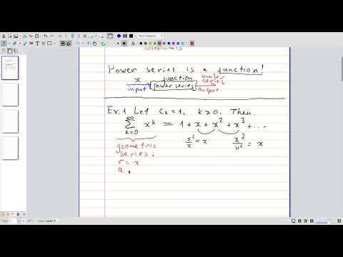
| 1 | Notes on power series | |
| 1.1 | Definition of power series The image quality is not great, and the colors are inverted. This has been corrected in subsequent videos |
 |
| 1.2 | Find the values of \(x\) that make the power series \(\sum_k \frac{(x-3)^k}k\) converge | 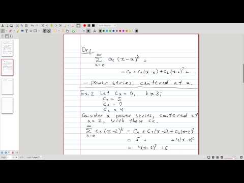 |
| 1.3 | Finding the regions of convergence for \(\sum_k k!x^k \) and the Bessel function \( J_0 \) | 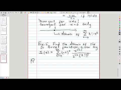 |
| 1.4 | We explore the graph of the Bessel function \( J_0 \) | 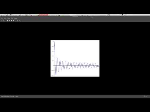 |
| 1.5 | Summary of different convergence modes for power series. | 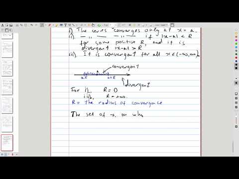 |
| 1.6 | Using the theorem from 1.5, we determine the interval of convergence (= all the values of \(x\) for which it converges) for the series \( \sum_k \frac{(-3)^k x^k}{\sqrt{k+1}} \). | 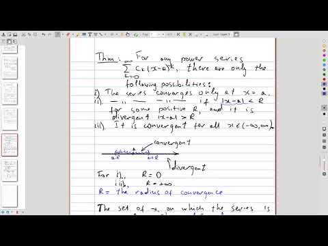 |
Representing functions by power series
| # | Topics | Links to video |
|---|---|---|
| 2 | Notes on representing functions by power series | |
| 2.1 | Representing functions with power series using algebraic manipulations | 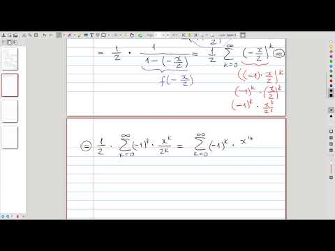 |
| 2.2 | The main theorem concerning differentiation and integration of power series, and an example that involves differentiating a series | 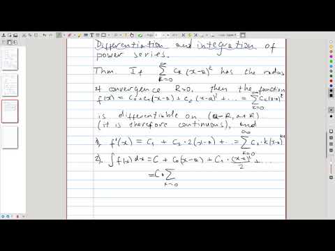 |
| 2.2a | A comment on changing indexing in a series | 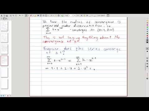 |
| 2.3 | Two important examples: power series for \(\ln(1+x)\) and \(\arctan x\) | 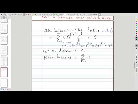 |
| 2.4 | Discussion of the series for \(\ln(1+x)\) and \(\arctan x\) | 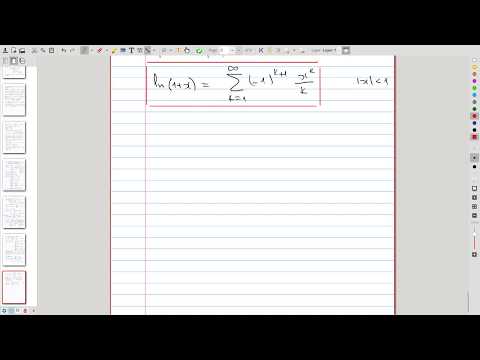 |
| 2.5 | Representing an antiderivative of a function by the power series and why it is useful | 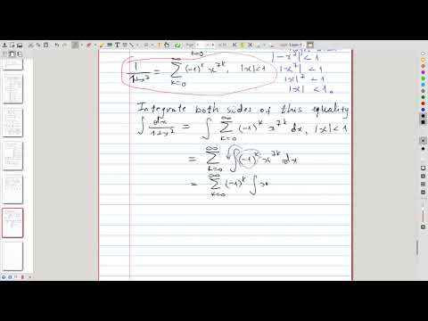 |
Bonus: A relation between power series and differential equations
| # | Topics | Links to video |
|---|---|---|
| A relation between power series and differential equations. | ||
| We solve the homework question #8 from section 11.9. First, we show that the power series \(f(x) = \sum_{n=0}^\infty \frac{x^n}{n!} \) satisfies the differential equation \(f’(x)=f(x)\). Then, we solve this differential equation and verify that its unique solution with the initial condition \(f(0)=1\) is \(e^x\). This gives an alternative way to compute the power series representation for \(e^x\). | 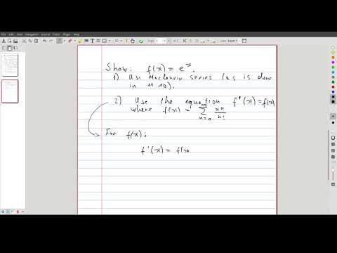 |
Taylor and Maclaurin series
| # | Topics | Links to video |
|---|---|---|
| 3 | Notes on Taylor and Maclaurin series | |
| 3.1 | The main theorem about Taylor series is discussed, which gives the expressions for the coefficients in the Taylor series of a function through its derivatives | 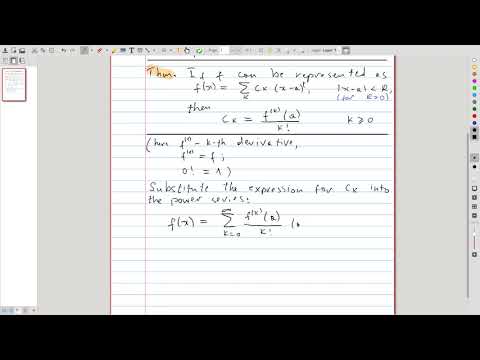 |
| 3.2 | Computing the Maclaurin series for \(e^x\) | 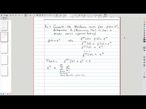 |
| 3.3 | How to prove that Taylor series of a function converges to it? We discuss the remainder estimate | 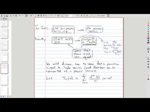 |
| 3.4 | Using the remainder estimate, we show that the Maclaurin series for \(e^x\) converges to it | 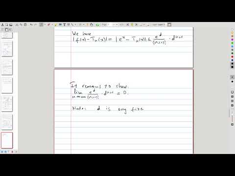 |
| 3.5 | Maclaurin series for \(\sin x\) | 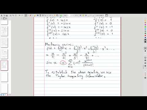 |
| 3.6 | Using the previous example, we calculate the Maclaurin expansion for \(\cos x\) | 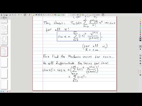 |
| 3.7 | We apply algebraic manipulations to the series for \(\cos x\) in order to compute the Maclaurin series of \(x \cos(x^3)\) and its radius of convergence | 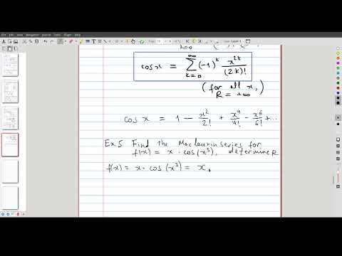 |
| 3.8 | The binomial series: expansion of \((1+x)^p\) | 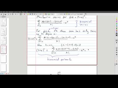 |
| 3.9 | Proof of the main theorem about Taylor series from 3.1 | 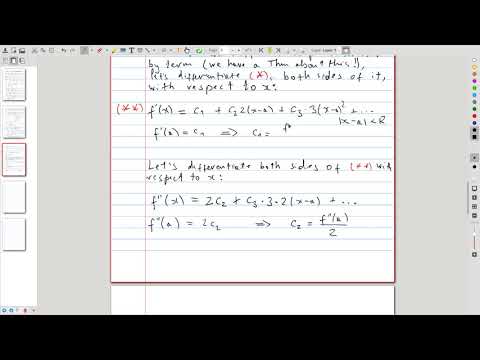 |
Additional examples and applications of Taylor and Maclaurin series
| # | Topics | Links to video |
|---|---|---|
| 3a | Notes on examples and applications of Taylor and Maclaurin series | |
| 3.10 | We consider an application of the binomial series formula, obtaining the Maclaurin expansion for \(\frac1{\sqrt{4-x}}\) | 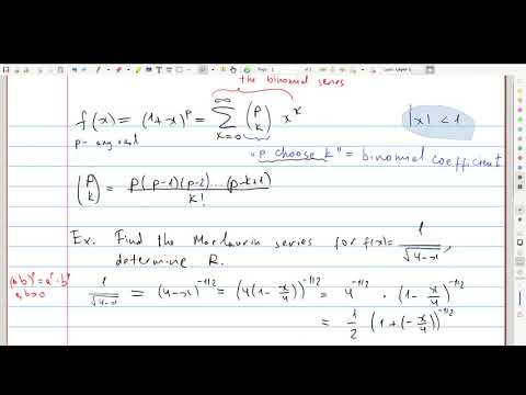 |
| 3.11 | An example of computing a Taylor series — the expansion of \(\sin x\) around the center \(a = \frac{\pi}{3}\) | 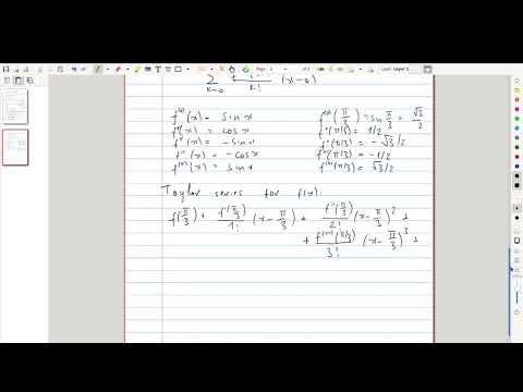 |
| 3.12 | Using power series to compute limits Turns out, not only power series can be used to approximate functions and compute antiderivatives, you can also use them instead of l’Hôpital’s rule to evaluate limits! |
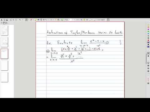 |
| 3.13 | Example of multiplying two power series We mentioned earlier that power series were the closest thing to infinite polynomials. In this video we show they are in fact so close to polynomials, one can multiply two power series together! |
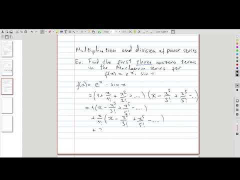 |
| 3.14 | Division of power series If the previous video was somewhat surprising, this one is nothing short of astounding. We will perform long division on infinite series, just like as if they were polynomials 😮 |
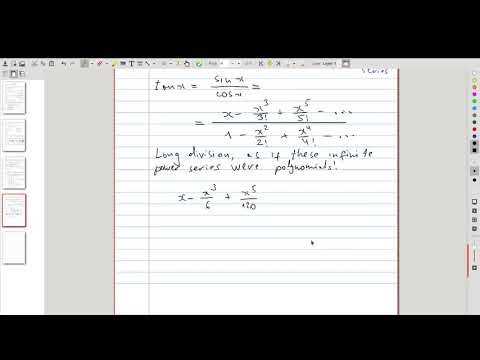 |
Approximating functions with Taylor polynomials
| # | Topics | Links to video |
|---|---|---|
| 4 | Notes on approximation with Taylor polynomials | |
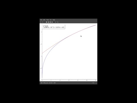
| 4.1 | Approximating \( \sqrt[3]x\) close to the point \(a = 8\) with \(T_2(x)\), and estimating the resulting error We discuss a typical application of Taylor series — approximation of a function close to a point where its value is known. This is how Taylor series usually show up in computational applications. |
 |
| 4.2 | Antiderivative of \( e^{-x^2} \) The antiderivative of \( e^{-x^2} \) cannot expressed in terms of elementary functions. It can, however, be represented by a (Maclaurin) power series converging everywhere. We obtain such representation, demonstrating the expressiveness of power series. |
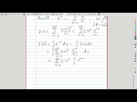 |
| 4.3 | Comparison of the initial Taylor polynomials We plot the function from episode 4.2 alongside several of its Taylor polynomials and discuss the code of the Python routine used to produce these graphs. |
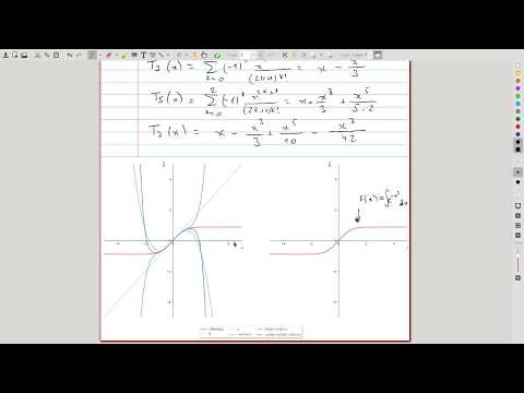 |
Parametric curves
| # | Topics | Links to video |
|---|---|---|
| 5 | Notes on parametric curves | |
| 5.1 | The definition of the parametric curve. Curve as a trajectory of motion | 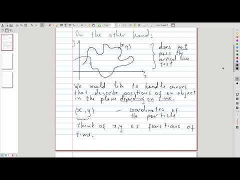 |
| 5.2 | Parameter elimination technique We introduce the primary technique for expressing a parametric curve as a regular curve: by eliminating the parameter \(t\). This technique is used to identify a parametric curve. |
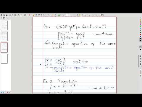 |
| 5.3 | The parametric curve \( (x(t),\, y(t)) = (t^2, \ln t) \) We show that every parametric curve has two characteristics: the shape and the direction of motion of a particle along this shape. Plus, in this example we get to reverse time Dr. Who-style 😮 |
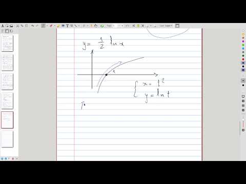 |
| 5.4 | The parametric curve \( (x(t),\, y(t)) = (\sin t, \sin^2 t) \) A piece of parabola along which we oscillate back and forth |
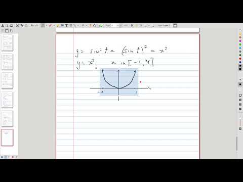 |
| 5.5 | The parametric curve \( (x(t),\, y(t)) = (\tan^2\theta, \sec \theta ) \), which shows that the range of the parameter is important | 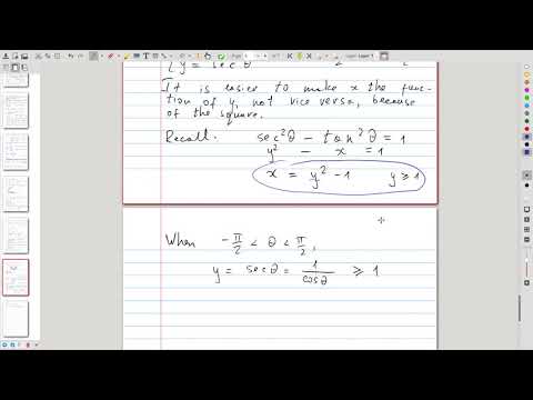 |
| 5.6 | Tangents to parametric curve We look at a self-intersecting curve, which has not one, but two tangents at the same point! (and does not pass the vertical line test) Link to SageMath. |
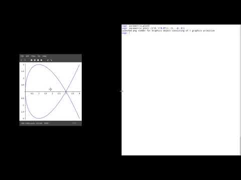 |
| 5.7 | Computing arc length of parametric curves The formula and an example: length of a circle |
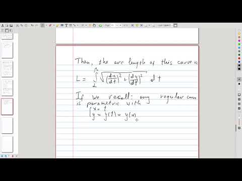 |
| 5.8 | Area of surfaces of revolution for parametric curves The formula and an example: area of a sphere |
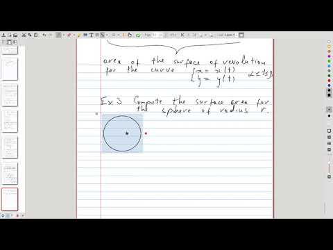 |
Polar coordinates and applications
| # | Topics | Links to video |
|---|---|---|
| 6 | Notes on polar coordinates and applications | |
| 6.1 | Definition of the polar coordinate system | 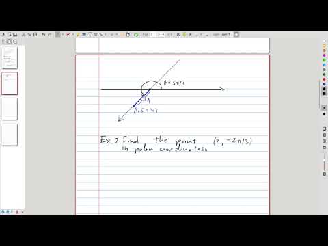 |
| 6.2 | Conversion formulas: converting between Cartesian and polar coordinates | 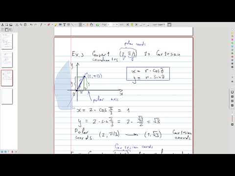 |
| 6.3 | Polar curves, definition and simple examples | 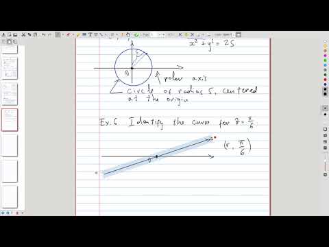 |
| 6.4 | Sketching polar curves, illustrated for the cardioid |  |
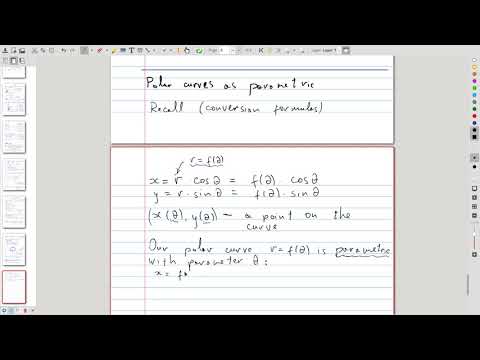
| 6.5 | Polar curves from the parametric perspective We treat polar curves as a special case of parametric curves and establish the formulas for slope and arc length of a polar curve This and the following video suffer from a nasty reverb 😞 |
 |
| 6.6 | To illustrate arc length formula for polar curves, we evaluate the length of the cardioid, which results in a tricky integral | 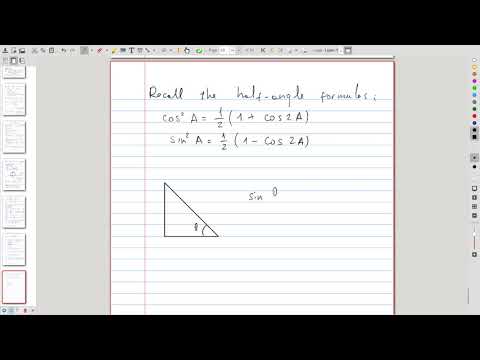 |
| Notes on areas in polar coordinates | ||
| 6.7 | Formula for computing areas in polar coordinates | 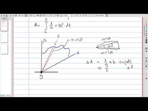 |
| 6.8 | An example for area in polar coordinates: the region inside the circle \(r = 3\sin \theta\) and outside the cardioid \(r = 1+\sin\theta\) | 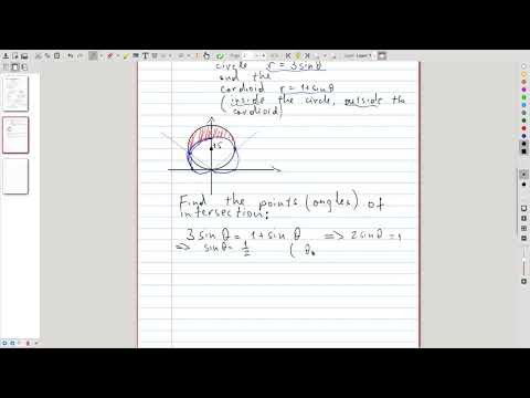 |
Conic sections
| # | Topics | Links to video |
|---|---|---|
| 7 | Notes on conic sections | |
| 7.1 | We discuss various conic sections and show how to obtain them by intersecting the double cone with a plane | 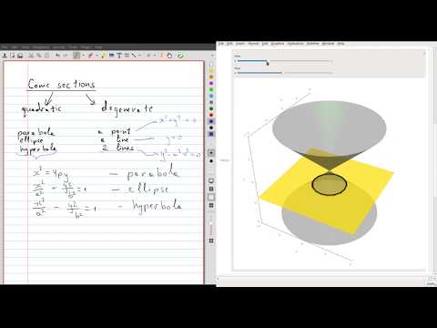 |
| 7.2 | Parabola: geometric characterization and equation | 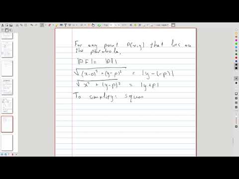 |
| 7.3 | Ellipse: geometric characterization and equation | 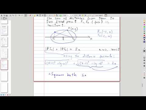 |
| 7.4 | Hyperbola: geometric characterization and equation | 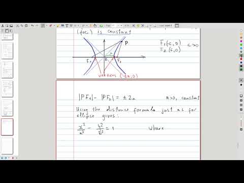 |